
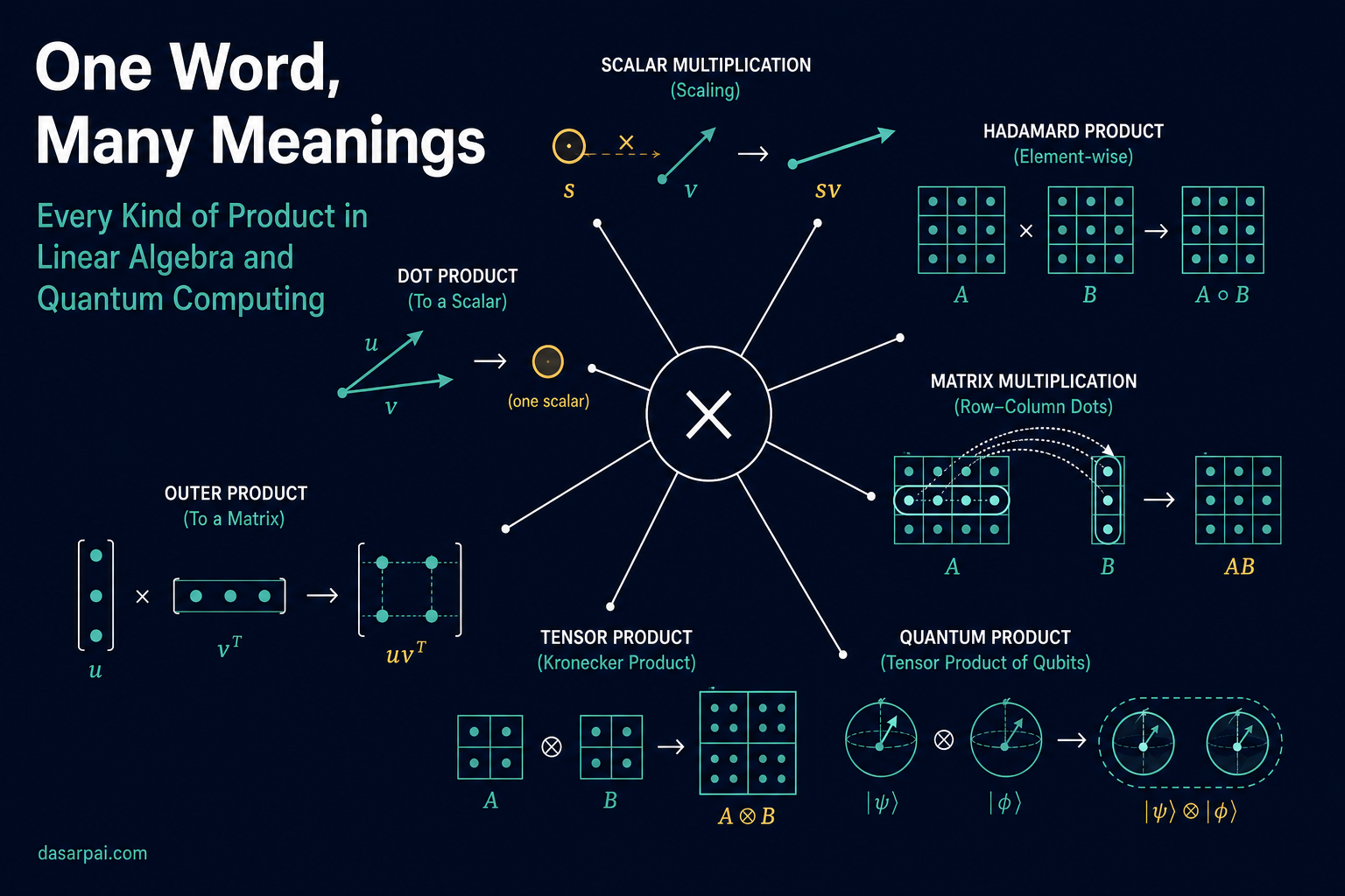
One Word, Many Meanings: Understanding Every Kind of Product in Linear Algebra and Quantum Computing#
Part 8 of the Learning Quantum Physics series. Parts 1–7 explored foundations, measurement, philosophy, and fields; from here the series adds the mathematical vocabulary used in quantum computing.
One of the first surprises students encounter while learning linear algebra, machine learning, or quantum computing is that the word product does not always mean the same thing.
In elementary arithmetic, multiplication seems straightforward:
\[ 3\times4=12 \]But once we begin working with vectors, matrices, and tensors, we encounter many different products:
- Scalar multiplication
- Pairwise operations
- Hadamard product
- Dot product
- Inner product
- Frobenius inner product
- Outer product
- Matrix–vector multiplication
- Matrix multiplication
- Cross product
- Tensor product
- Kronecker product
Naturally, a beginner may wonder:
Why do we need so many different ways of multiplying?
The answer is surprisingly simple:
Each product combines mathematical objects for a different purpose and produces a different kind of result.
Some products produce a scalar. Some preserve the original shape. Some construct a matrix. Some apply a transformation. Others combine entire physical systems.
To understand them clearly, we must always ask four questions:
- What kinds of objects are being combined?
- How are their elements matched?
- Are the resulting products retained or added?
- What type of object comes out?
1. First, What Are Scalars, Vectors, Matrices, and Tensors?#
Before discussing products, we should identify the objects being multiplied.
Scalar#
A scalar is one number:
\[ c=5 \]Vector#
A vector is a one-dimensional sequence of numbers:
\[ \mathbf u= \begin{bmatrix} 1\\ 2 \end{bmatrix} \]Its shape is \(2\times1\) when written as a column vector.
Matrix#
A matrix is a two-dimensional arrangement of numbers:
\[ A= \begin{bmatrix} 1&2\\ 3&4 \end{bmatrix} \]Its shape is \(2\times2\).
Tensor#
A tensor is the general multidimensional idea.
From the computational perspective:
- Scalar: zero-dimensional tensor
- Vector: one-dimensional tensor
- Matrix: two-dimensional tensor
- 3D array: third-order tensor
- Higher-dimensional array: higher-order tensor
There is more mathematical depth behind the word tensor, but this understanding is sufficient for our present discussion.
2. Scalar Multiplication#
Scalar multiplication means multiplying every element of a vector, matrix, or tensor by one scalar.
Suppose:
\[ c=5, \qquad \mathbf u= \begin{bmatrix} 1\\ 2 \end{bmatrix} \]Then:
\[ \begin{aligned} c\mathbf u \\ &= 5 \begin{bmatrix} 1\\ 2 \end{bmatrix} \\ &= \begin{bmatrix} 5\\ 10 \end{bmatrix} \end{aligned} \]The same operation can be applied to a matrix:
\[ \begin{aligned} 5 \begin{bmatrix} 1&2\\ 3&4 \end{bmatrix} \\ &= \begin{bmatrix} 5&10\\ 15&20 \end{bmatrix} \end{aligned} \]Output#
The output has the same shape as the original object.
Meaning#
Scalar multiplication answers:
What happens if I scale every component of this object by the same amount?
For vectors:
- Multiplication by \(5\) makes the vector five times longer.
- Multiplication by \(0.5\) makes it half as long.
- Multiplication by a negative number also reverses its direction.
- Multiplication by zero produces the zero vector.
Scalar multiplication versus scalar product#
These terms should not be confused.
- Scalar multiplication means scalar × vector, matrix, or tensor.
- Scalar product is sometimes used as another name for the dot product or inner product because its output is a scalar.
The phrase scalar product is therefore potentially confusing. It is better to use the more precise terms scalar multiplication, dot product, or inner product.
3. Pairwise Operations#
Pairwise, or element-wise, is not the name of one particular product.
It describes how elements are matched:
An element in one object is paired with the element at the same position in the other object.
Consider:
\[ A= \begin{bmatrix} 1&2\\ 3&4 \end{bmatrix}, \qquad B= \begin{bmatrix} 5&2\\ 1&8 \end{bmatrix} \]The corresponding pairs are:
\[ (1,5),\quad(2,2),\quad(3,1),\quad(4,8) \]We can apply many operations to these pairs.
Pairwise addition#
\[ \begin{aligned} A+B \\ &= \begin{bmatrix} 1+5&2+2\\ 3+1&4+8 \end{bmatrix} \\ &= \begin{bmatrix} 6&4\\ 4&12 \end{bmatrix} \end{aligned} \]Pairwise subtraction#
\[ \begin{aligned} A-B \\ &= \begin{bmatrix} -4&0\\ 2&-4 \end{bmatrix} \end{aligned} \]Pairwise division#
\[ \begin{aligned} A\oslash B \\ &= \begin{bmatrix} 1/5&2/2\\ 3/1&4/8 \end{bmatrix} \\ &= \begin{bmatrix} 0.2&1\\ 3&0.5 \end{bmatrix} \end{aligned} \]Division fails wherever the corresponding element in (B) is zero.
Pairwise comparison#
\[ \begin{aligned} A>B \\ &= \begin{bmatrix} 1>5&2>2\\ 3>1&4>8 \end{bmatrix} \end{aligned} \]Therefore:
\[ \begin{aligned} A>B \\ &= \begin{bmatrix} \text{False}&\text{False}\\ \text{True}&\text{False} \end{bmatrix} \end{aligned} \]Other pairwise operations include:
- Equality and inequality
- Maximum and minimum
- Powers
- Remainders
- Logical AND and OR
- Absolute differences
The general form is:
\[ C_{ij}=f(A_{ij},B_{ij}) \]where (f) may be addition, multiplication, comparison, or any other suitable two-input operation.
Pairwise operations can be performed on:
- Vectors
- Matrices
- 3D tensors
- Higher-dimensional tensors
Normally, the two objects must have the same shape. Programming libraries may also permit compatible shapes through broadcasting, but broadcasting adds an extra rule; it is not simply ordinary same-position pairing.
4. Hadamard Product#
The Hadamard product is specifically pairwise multiplication.
Symbol#
\[ A\odot B \]Consider:
\[ A= \begin{bmatrix} 1&2\\ 3&4 \end{bmatrix}, \qquad B= \begin{bmatrix} 5&6\\ 7&8 \end{bmatrix} \]Then:
\[ \begin{aligned} A\odot B \\ &= \begin{bmatrix} 1(5)&2(6)\\ 3(7)&4(8) \end{bmatrix} \\ &= \begin{bmatrix} 5&12\\ 21&32 \end{bmatrix} \end{aligned} \]Output#
A matrix with the same shape as the inputs.
The Hadamard product also applies to vectors and tensors of any dimension:
\[ \begin{aligned} (A\odot B)_{i_1i_2\ldots i_k} \\ &= A_{i_1i_2\ldots i_k} B_{i_1i_2\ldots i_k} \end{aligned} \]Meaning#
The Hadamard product answers:
What do I get if I multiply corresponding elements while retaining every individual result?
This gives us an important distinction:
\[ \boxed{\text{Pairwise operation}=\text{general category}} \]\[ \boxed{\text{Hadamard product}=\text{pairwise multiplication}} \]Therefore, every Hadamard product is a pairwise operation, but not every pairwise operation is a Hadamard product.
5. Dot Product#
The dot product is normally defined between two equal-length vectors.
Consider:
\[ \mathbf u= \begin{bmatrix} 1\\ 2 \end{bmatrix}, \qquad \mathbf v= \begin{bmatrix} 3\\ 4 \end{bmatrix} \]Symbols#
\[ \mathbf u\cdot\mathbf v \]or:
\[ \mathbf u^T\mathbf v \]First multiply the corresponding components:
\[ \begin{aligned} \mathbf u\odot\mathbf v \\ &= \begin{bmatrix} 1(3)\\ 2(4) \end{bmatrix} \\ &= \begin{bmatrix} 3\\ 8 \end{bmatrix} \end{aligned} \]Then add the products:
\[ 3+8=11 \]Therefore:
\[ \mathbf u\cdot\mathbf v=11 \]In general:
\[ \begin{aligned} \mathbf u\cdot\mathbf v = \sum_{i=1}^{n} u_i v_i \end{aligned} \]Output#
One scalar.
Meaning#
The dot product answers:
How strongly does one vector point in the direction of the other?
Geometrically:
\[ \begin{aligned} \mathbf u\cdot\mathbf v = |\mathbf u||\mathbf v|\cos\theta \end{aligned} \]where:
- \(\|\mathbf u\|\) is the length of \(\mathbf u\)
- \(\|\mathbf v\|\) is the length of \(\mathbf v\)
- \(\theta\) is the angle between them
Therefore:
- Positive result: broadly aligned
- Zero: perpendicular or orthogonal
- Negative result: broadly opposite
Hadamard versus dot product#
Both begin with corresponding-element multiplication.
The difference is what happens next:
\[ \begin{aligned} \mathbf u\odot\mathbf v = \begin{bmatrix} 3\\ 8 \end{bmatrix} \end{aligned} \]The Hadamard product retains the individual products.
But:
\[ \mathbf u\cdot\mathbf v=3+8=11 \]The dot product adds them and returns one scalar.
Thus:
\[ \boxed{\text{Dot product}=\text{Hadamard product followed by total summation}} \]for two equal-length real vectors.
6. Inner Product#
The inner product is the broader mathematical concept. The dot product is one particular inner product.
General notation#
\[ \langle\mathbf u,\mathbf v\rangle \]For ordinary real vectors using the standard inner product:
\[ \begin{aligned} \langle\mathbf u,\mathbf v\rangle \\ &= \mathbf u^T\mathbf v \\ &= \mathbf u\cdot\mathbf v \end{aligned} \]Therefore, in an ordinary real vector space:
\[ \boxed{\text{Dot product}=\text{standard inner product}} \]The inner product is not limited to quantum mechanics or complex vectors. It is a general rule that allows us to define:
- Length
- Angle
- Orthogonality
- Projection
- Similarity
For example, vector length is derived from:
\[ \begin{aligned} |\mathbf u| = \sqrt{\langle\mathbf u,\mathbf u\rangle} \end{aligned} \]Two vectors are orthogonal when:
\[ \langle\mathbf u,\mathbf v\rangle=0 \]Complex inner product#
When vectors contain complex numbers, one vector must be complex-conjugated.
Consider:
\[ \mathbf u= \begin{bmatrix} 1\\ i \end{bmatrix}, \qquad \mathbf v= \begin{bmatrix} 2\\ 3i \end{bmatrix} \]The conjugate transpose of \(\mathbf u\) is:
\[ \mathbf u^\dagger= \begin{bmatrix} 1&-i \end{bmatrix} \]Then:
\[ \begin{aligned} \langle\mathbf u,\mathbf v\rangle = \mathbf u^\dagger\mathbf v \end{aligned} \]\[ 1(2)+(-i)(3i) \]Since \(i^2=-1\):
\[ (-i)(3i)=-3i^2=3 \]Therefore:
\[ \langle\mathbf u,\mathbf v\rangle=2+3=5 \]The conjugation ensures that the inner product of a vector with itself is a real, non-negative number:
\[ \begin{aligned} \langle\mathbf u,\mathbf u\rangle = \mathbf u^\dagger\mathbf u \ge 0 \end{aligned} \]7. Inner Product in Dirac Notation#
Quantum mechanics commonly uses Dirac’s bra–ket notation.
A column vector is written as a ket:
\[ |\psi\rangle \]Its conjugate transpose is written as a bra:
\[ \langle\psi| \]The inner product between two quantum states is:
\[ \langle\psi|\phi\rangle \]Ordinary mathematical notation writes:
\[ \langle\psi,\phi\rangle \]Dirac notation writes:
\[ \langle\psi|\phi\rangle \]The two notations express the same underlying inner-product idea.
The inner product produces a scalar, generally called a probability amplitude in quantum mechanics. Its squared magnitude gives a probability:
\[ P=|\langle\psi|\phi\rangle|^2 \]So it is more precise to say:
An inner product measures overlap between quantum states; the squared magnitude of that overlap gives the relevant probability.
8. Frobenius Inner Product#
We normally use the term dot product for vectors. When the same idea is applied to two same-shaped matrices, it is called the Frobenius inner product.
Consider:
\[ A= \begin{bmatrix} 1&2\\ 3&4 \end{bmatrix}, \qquad B= \begin{bmatrix} 5&6\\ 7&8 \end{bmatrix} \]First calculate the Hadamard product:
\[ \begin{aligned} A\odot B = \begin{bmatrix} 5&12\\ 21&32 \end{bmatrix} \end{aligned} \]Then add every element:
\[ 5+12+21+32=70 \]Therefore:
\[ \langle A,B\rangle_F=70 \]The subscript (F) means Frobenius.
For real matrices:
\[ \begin{aligned} \langle A,B\rangle_F = \sum_{i,j} A_{ij}\, B_{ij} \end{aligned} \]It can also be written as:
\[ \begin{aligned} \langle A,B\rangle_F = \operatorname{tr}(A^TB) \end{aligned} \]where (\operatorname{tr}) means the sum of the diagonal elements.
Why does this resemble a dot product?#
Because it is exactly the dot product of the flattened matrices.
Flatten (A) and (B):
\[ \operatorname{vec}(A)= \begin{bmatrix} 1\\2\\3\\4 \end{bmatrix}, \qquad \operatorname{vec}(B)= \begin{bmatrix} 5\\6\\7\\8 \end{bmatrix} \]Then:
\[ \begin{aligned} \operatorname{vec}(A)\cdot\operatorname{vec}(B) \\ &= 1(5)+2(6)+3(7)+4(8) =70 \end{aligned} \]Thus:
\[ \boxed{\langle A,B\rangle_F=\operatorname{vec}(A)\cdot\operatorname{vec}(B)} \]The separate name is useful because the original inputs are matrices.
For complex matrices, the conjugate transpose is required:
\[ \begin{aligned} \langle A,B\rangle_F = \operatorname{tr}(A^\dagger B) \end{aligned} \]9. Full Inner Product of Tensors#
The same idea extends to same-shaped higher-dimensional tensors.
For two 3D tensors (X) and (Y):
\[ \begin{aligned} \langle X,Y\rangle = \sum_{i,j,k} X_{ijk}\, Y_{ijk} \end{aligned} \]This means:
- Multiply corresponding elements.
- Sum over every dimension.
- Produce one scalar.
It may be called:
- Tensor inner product
- Full tensor contraction
- Frobenius inner product of tensors
The complete pattern is now visible:
| Inputs | Common name | Procedure | Output |
|---|---|---|---|
| Two vectors | Dot product | Multiply corresponding elements and sum | Scalar |
| Two matrices | Frobenius inner product | Multiply corresponding elements and sum | Scalar |
| Two same-shaped tensors | Full tensor inner product | Multiply corresponding elements and sum | Scalar |
All three apply the same essential idea to differently shaped objects.
10. Outer Product#
The outer product reverses the shape arrangement used in the vector inner product.
Consider:
\[ \mathbf u= \begin{bmatrix} 1\\ 2 \end{bmatrix}, \qquad \mathbf v= \begin{bmatrix} 3\\ 4 \end{bmatrix} \]The inner product is:
\[ \mathbf u^T\mathbf v \]Its shapes are:
\[ (1\times2)(2\times1) \rightarrow 1\times1 \]It produces a scalar.
The outer product is:
\[ \mathbf u\mathbf v^T \]Its shapes are:
\[ (2\times1)(1\times2) \rightarrow 2\times2 \]Calculating it:
\[ \begin{aligned} \mathbf u\mathbf v^T \\ &= \begin{bmatrix} 1\\ 2 \end{bmatrix} \begin{bmatrix} 3&4 \end{bmatrix} \end{aligned} \]\[ \begin{aligned} \begin{bmatrix} 1(3)&1(4)\\ 2(3)&2(4) \end{bmatrix} \\ &= \begin{bmatrix} 3&4\\ 6&8 \end{bmatrix} \end{aligned} \]Output#
A matrix.
Meaning#
The outer product answers:
What matrix can be constructed by combining every component of one vector with every component of the other?
In quantum computing, outer products are written as:
\[ |\psi\rangle\langle\phi| \]They are used to construct:
- Projection operators
- Density matrices
- State-transition operators
- Measurement operators
For example:
\[ |0\rangle= \begin{bmatrix} 1\\0 \end{bmatrix} \]Then:
\[ \begin{aligned} |0\rangle\langle0| \\ &= \begin{bmatrix} 1\\0 \end{bmatrix} \begin{bmatrix} 1&0 \end{bmatrix} \\ &= \begin{bmatrix} 1&0\\ 0&0 \end{bmatrix} \end{aligned} \]This matrix projects a quantum state onto the \(|0\rangle\) direction.
Inner versus outer product#
\[ \boxed{\langle\mathbf u,\mathbf v\rangle \rightarrow \text{scalar measuring overlap}} \]\[ \boxed{\mathbf u\mathbf v^T \rightarrow \text{matrix constructed from the vectors}} \]The word inner suggests that dimensions are contracted into a scalar. The word outer suggests that the result expands into a matrix.
11. Matrix–Vector Multiplication#
A matrix commonly represents a linear transformation, while a vector represents an input or state.
Consider:
\[ A= \begin{bmatrix} 2&0\\ 0&3 \end{bmatrix}, \qquad \mathbf x= \begin{bmatrix} 5\\ 4 \end{bmatrix} \]Then:
\[ \begin{aligned} A\mathbf x \\ &= \begin{bmatrix} 2(5)+0(4)\\ 0(5)+3(4) \end{bmatrix} \\ &= \begin{bmatrix} 10\\ 12 \end{bmatrix} \end{aligned} \]Output#
A vector.
Meaning#
Matrix–vector multiplication answers:
What does this transformation do to this vector?
Each output component is the dot product of:
- One row of the matrix
- The input vector
For example:
\[ \begin{bmatrix} 2&0 \end{bmatrix} \cdot \begin{bmatrix} 5\\4 \end{bmatrix} =10 \]In this example, (A):
- Multiplies the first coordinate by \(2\)
- Multiplies the second coordinate by \(3\)
In quantum computing:
\[ X|0\rangle=|1\rangle \]is matrix–vector multiplication. The \(X\) gate is a matrix, and \(|0\rangle\) is the state vector.
12. Matrix Multiplication#
Matrix multiplication combines two linear transformations.
Consider:
\[ A= \begin{bmatrix} 1&2\\ 3&4 \end{bmatrix}, \qquad B= \begin{bmatrix} 5&6\\ 7&8 \end{bmatrix} \]Then:
\[ \begin{aligned} AB &= \begin{bmatrix} 1(5)+2(7)&1(6)+2(8)\\ 3(5)+4(7)&3(6)+4(8) \end{bmatrix} \end{aligned} \]Therefore:
\[ AB= \begin{bmatrix} 19&22\\ 43&50 \end{bmatrix} \]Every output element is the dot product of:
- One row of (A)
- One column of (B)
For example:
\[ \begin{aligned} (AB)_{11} \\ &= \begin{bmatrix} 1&2 \end{bmatrix} \cdot \begin{bmatrix} 5\\7 \end{bmatrix} =19 \end{aligned} \]Thus:
Matrix multiplication is a structured collection of row–column dot products.
However, the complete operation produces a matrix, not one scalar.
Shape rule#
If:
\[ A\in\mathbb R^{m\times n} \]and:
\[ B\in\mathbb R^{n\times p} \]then:
\[ AB\in\mathbb R^{m\times p} \]The inner dimensions must match:
\[ \begin{aligned} (m\times\boxed n)(\boxed n\times p) \\ &= m\times p \end{aligned} \]Interpretation#
Suppose:
- (B) rotates a vector.
- (A) stretches the rotated vector.
Then:
\[ \begin{aligned} AB\mathbf x = A(B\mathbf x) \end{aligned} \]This means:
- Apply (B) first.
- Apply (A) second.
Therefore, (AB) represents the composition of two transformations.
Matrix multiplication versus Hadamard multiplication#
Using the same matrices:
\[ A\odot B= \begin{bmatrix} 5&12\\ 21&32 \end{bmatrix} \]But:
\[ AB= \begin{bmatrix} 19&22\\ 43&50 \end{bmatrix} \]They are entirely different operations:
- Hadamard multiplication pairs corresponding elements.
- Matrix multiplication takes row–column dot products.
13. Cross Product#
The cross product is usually defined for two 3D vectors.
Consider:
\[ \mathbf a= \begin{bmatrix} 1\\0\\0 \end{bmatrix}, \qquad \mathbf b= \begin{bmatrix} 0\\1\\0 \end{bmatrix} \]Then:
\[ \begin{aligned} \mathbf a\times\mathbf b = \begin{bmatrix} 0\\0\\1 \end{bmatrix} \end{aligned} \]Output#
A vector perpendicular to both input vectors.
For general 3D vectors:
\[ \mathbf a= \begin{bmatrix} a_1 \\ a_2 \\ a_3 \end{bmatrix}, \qquad \mathbf b= \begin{bmatrix} b_1 \\ b_2 \\ b_3 \end{bmatrix} \]the cross product is:
\[ \begin{aligned} \mathbf a\times\mathbf b = \begin{bmatrix} a_2b_3-a_3b_2\\ a_3b_1-a_1b_3\\ a_1b_2-a_2b_1 \end{bmatrix} \end{aligned} \]Its magnitude is:
\[ \begin{aligned} |\mathbf a\times\mathbf b| = |\mathbf a||\mathbf b|\sin\theta \end{aligned} \]This magnitude equals the area of the parallelogram formed by the two vectors.
Meaning#
The cross product answers:
Which vector is perpendicular to both input vectors, and what oriented area do they form?
The direction is determined by the right-hand rule.
The order matters:
\[ \begin{aligned} \mathbf a\times\mathbf b = -(\mathbf b\times\mathbf a) \end{aligned} \]Therefore, the cross product is not commutative.
Dot versus cross product#
| Property | Dot product | Cross product |
|---|---|---|
| Symbol | (\mathbf a\cdot\mathbf b) | (\mathbf a\times\mathbf b) |
| Output | Scalar | Vector |
| Geometric factor | (\cos\theta) | (\sin\theta) |
| Zero when | Vectors are perpendicular | Vectors are parallel |
| Main meaning | Alignment | Perpendicular direction and area |
14. Tensor Product#
The tensor product combines two mathematical spaces or physical systems into one larger composite space.
Symbol#
\[ \mathbf u\otimes\mathbf v \]Using:
\[ \mathbf u= \begin{bmatrix} 1\\ 2 \end{bmatrix}, \qquad \mathbf v= \begin{bmatrix} 3\\ 4 \end{bmatrix} \]we obtain:
\[ \begin{aligned} \mathbf u\otimes\mathbf v \\ &= \begin{bmatrix} 1(3)\\ 1(4)\\ 2(3)\\ 2(4) \end{bmatrix} \\ &= \begin{bmatrix} 3\\ 4\\ 6\\ 8 \end{bmatrix} \end{aligned} \]If:
\[ \mathbf u\in\mathbb R^m, \qquad \mathbf v\in\mathbb R^n \]then:
\[ \mathbf u\otimes\mathbf v\in\mathbb R^{mn} \]Output#
A larger vector representing the combined space.
Meaning#
The tensor product answers:
How do I represent two systems together as one composite system?
This is fundamental in quantum computing.
For one qubit:
\[ |0\rangle= \begin{bmatrix} 1\\0 \end{bmatrix}, \qquad |1\rangle= \begin{bmatrix} 0\\1 \end{bmatrix} \]For two qubits:
\[ \begin{aligned} |0\rangle\otimes|1\rangle \\ &= |01\rangle \end{aligned} \]Numerically:
\[ \begin{aligned} \begin{bmatrix} 1\\0 \end{bmatrix} \otimes \begin{bmatrix} 0\\1 \end{bmatrix} \\ &= \begin{bmatrix} 0\\1\\0\\0 \end{bmatrix} \end{aligned} \]The two-qubit state space contains four basis states:
\[ |00\rangle,\quad|01\rangle,\quad|10\rangle,\quad|11\rangle \]This is why:
- One qubit requires \(2\) amplitudes.
- Two qubits require \(4\) amplitudes.
- Three qubits require \(8\) amplitudes.
- \(n\) qubits require \(2^n\) amplitudes.
An important refinement is that tensor products combine systems into a composite system. The systems may initially be independent, but the combined space also allows entangled states, which cannot be separated into individual tensor factors.
15. Kronecker Product#
When tensor products of matrices are calculated in coordinates, the operation is commonly represented by the Kronecker product.
It uses the same symbol:
\[ A\otimes B \]Suppose:
\[ A= \begin{bmatrix} a&b\\ c&d \end{bmatrix} \]Then:
\[ \begin{aligned} A\otimes B \\ &= \begin{bmatrix} aB&bB\\ cB&dB \end{bmatrix} \end{aligned} \]Each element of (A) multiplies the entire matrix (B).
If (A) is (m\times n) and (B) is (p\times q), then:
\[ A\otimes B \]has shape:
\[ (mp)\times(nq) \]In quantum computing, if (H) is applied to the first qubit and (I) to the second, the combined operator is:
\[ H\otimes I \]Therefore:
- Tensor product is the general mathematical construction.
- Kronecker product is its common coordinate or block-matrix realization.
16. Outer Product versus Tensor Product#
For vectors, the outer product and tensor product contain the same pairwise multiplicative combinations, which can make them look almost identical.
Using:
\[ \mathbf u= \begin{bmatrix} 1\\2 \end{bmatrix}, \qquad \mathbf v= \begin{bmatrix} 3\\4 \end{bmatrix} \]the outer product is:
\[ \begin{aligned} \mathbf u\mathbf v^T = \begin{bmatrix} 3&4\\ 6&8 \end{bmatrix} \end{aligned} \]The tensor product is:
\[ \begin{aligned} \mathbf u\otimes\mathbf v = \begin{bmatrix} 3\\4\\6\\8 \end{bmatrix} \end{aligned} \]Both contain:
\[ 3,\quad4,\quad6,\quad8 \]But their meanings and representations differ:
- The outer product is represented as a matrix and commonly acts as an operator.
- The tensor product represents an element of a combined space.
- With a chosen ordering convention, one can be reshaped into the other.
- The tensor-product concept extends naturally to composite systems and higher-order objects.
So they are closely related, but they answer different questions.
17. Contraction: The Hidden Idea Behind Many Products#
We can now see a deeper pattern.
Suppose two objects contain compatible dimensions. A contraction means:
- Multiply along selected matching dimensions.
- Sum over those dimensions.
The vector dot product contracts the only dimension:
\[ \begin{aligned} \mathbf u\cdot\mathbf v = \sum_i u_iv_i \end{aligned} \]The Frobenius inner product contracts both matrix dimensions:
\[ \begin{aligned} \langle A,B\rangle_F = \sum_{i,j} A_{ij}\, B_{ij} \end{aligned} \]Matrix multiplication contracts one dimension:
\[ \begin{aligned} (AB)_{ij} = \sum_k A_{ik} B_{kj} \end{aligned} \]A full tensor inner product contracts every dimension:
\[ \begin{aligned} \langle X,Y\rangle \\ &= \sum_{i,j,k,\ldots} X_{ijk\ldots}\, Y_{ijk\ldots} \end{aligned} \]This explains why similar multiplication-and-summation patterns appear in several apparently different operations.
The difference is:
Which dimensions are multiplied and summed, and which dimensions remain in the output?
18. The Complete Comparison#
| Operation | Typical input | Procedure | Output | Main question |
|---|---|---|---|---|
| Scalar multiplication | Scalar × vector/matrix/tensor | Multiply every element by one number | Same-shaped object | How do I scale this object? |
| Pairwise operation | Same-shaped objects | Apply an operation to corresponding elements | Same-shaped object | What happens at each position? |
| Hadamard product | Same-shaped objects | Multiply corresponding elements | Same-shaped object | What are the individual pairwise products? |
| Dot product | Vector × vector | Multiply corresponding elements and sum | Scalar | How aligned are these vectors? |
| Inner product | Two elements of an inner-product space | Apply the space’s inner-product rule | Scalar | What are their overlap, angle, or orthogonality? |
| Frobenius inner product | Matrix × matrix | Multiply corresponding elements and sum all | Scalar | What is the overall matrix overlap? |
| Full tensor inner product | Same-shaped tensors | Multiply corresponding elements and sum all | Scalar | What is the overall tensor overlap? |
| Outer product | Vector × vector | Multiply every element with every other element | Matrix | What operator or matrix can these vectors construct? |
| Matrix–vector multiplication | Matrix × vector | Row–vector dot products | Vector | How does this transformation change the vector? |
| Matrix multiplication | Matrix × matrix | Row–column dot products | Matrix | What is the composition of these transformations? |
| Cross product | 3D vector × 3D vector | Special antisymmetric combination | 3D vector | What vector is perpendicular to both? |
| Tensor product | Two vectors/spaces/systems | Form all combined basis combinations | Larger object | How do I represent a composite system? |
| Kronecker product | Matrix × matrix | Replace every element of one matrix with a scaled copy of the other | Larger matrix | How do I represent a combined operator? |
19. A Compact Numerical Comparison#
Let:
\[ \mathbf u= \begin{bmatrix} 1\\2 \end{bmatrix}, \qquad \mathbf v= \begin{bmatrix} 3\\4 \end{bmatrix} \]Then:
Hadamard product#
\[ \begin{aligned} \mathbf u\odot\mathbf v = \begin{bmatrix} 3\\8 \end{bmatrix} \end{aligned} \]Corresponding products are retained.
Dot product#
\[ \begin{aligned} \mathbf u\cdot\mathbf v = 3+8=11 \end{aligned} \]Corresponding products are summed.
Outer product#
\[ \begin{aligned} \mathbf u\mathbf v^T = \begin{bmatrix} 3&4\\6&8 \end{bmatrix} \end{aligned} \]Every component of \(\mathbf u\) is combined with every component of \(\mathbf v\), and the result is arranged as a matrix.
Tensor product#
\[ \begin{aligned} \mathbf u\otimes\mathbf v \\ &= \begin{bmatrix} 3\\4\\6\\8 \end{bmatrix} \end{aligned} \]Every component is again combined with every other component, but the result represents a vector in a composite space.
The numbers overlap, but the structure and purpose change.
20. The Most Important Memory Map#
The entire discussion can be remembered through a few central patterns.
Corresponding elements are paired#
\[ C_{ij}=f(A_{ij},B_{ij}) \]This is a pairwise operation.
Corresponding elements are multiplied and retained#
\[ A\odot B \]This is the Hadamard product.
Corresponding vector elements are multiplied and summed#
\[ \begin{aligned} \mathbf u\cdot\mathbf v = \sum_i u_iv_i \end{aligned} \]This is the dot product.
Corresponding matrix elements are multiplied and summed#
\[ \begin{aligned} \langle A,B\rangle_F = \sum_{i,j} A_{ij}\, B_{ij} \end{aligned} \]This is the Frobenius inner product.
A matrix row and a vector are dotted#
\[ A\mathbf x \]This applies a transformation to a vector.
Matrix rows and columns are dotted#
\[ AB \]This composes transformations.
Every vector element is multiplied by every other vector element#
\[ \mathbf u\mathbf v^T \]This produces an outer-product matrix.
Two spaces or systems are combined#
\[ \mathbf u\otimes\mathbf v \]This produces a tensor-product space.
The Big Picture#
The various products of linear algebra are not different merely because mathematicians invented different symbols.
They exist because they answer fundamentally different questions:
- Scalar multiplication asks: How should this object be scaled?
- Pairwise operations ask: What happens at each corresponding position?
- Hadamard product asks: What are the corresponding element products?
- Dot product asks: How aligned are these vectors?
- Inner product asks: What are the overlap, length, angle, and orthogonality in this space?
- Frobenius inner product asks: What is the total overlap between these matrices?
- Outer product asks: What matrix or operator can these vectors construct?
- Matrix–vector multiplication asks: How does this transformation change this state?
- Matrix multiplication asks: What happens when transformations are composed?
- Cross product asks: What vector is perpendicular to both input vectors?
- Tensor product asks: How do we represent multiple systems together?
- Kronecker product asks: How do we write combined transformations as concrete matrices?
I think the deeper lesson is this:
Multiplication is not merely an arithmetic action. It is a rule for combining mathematical objects while preserving the particular relationship we want to study.
Sometimes we want to preserve every individual result. Sometimes we want to sum them into one scalar. Sometimes we want to construct a transformation. Sometimes we want to combine entire systems.
The numbers may be the same.
The multiplication signs may look similar.
But the mathematical question changes—and therefore, the meaning of the product changes.
Hashtags#
#LinearAlgebra #MachineLearning #QuantumComputing #DotProduct #MatrixMultiplication #TensorProduct #AppliedMathematics #DataScience #MathForML #InnerProduct

Comments: