
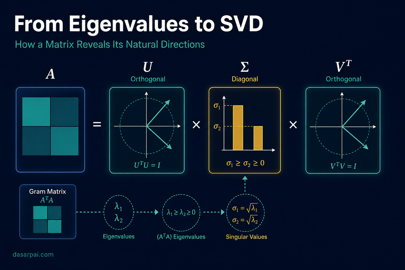
From Eigenvalues to Singular Value Decomposition#
How a matrix reveals its natural directions, strengths, and hidden simplicity#
Part 9 of the Learning Quantum Physics series.
Suppose we are given a matrix:
\[ M= \begin{bmatrix} 4&0\\ 3&-5 \end{bmatrix}. \]At first sight, it is only a rectangular arrangement of four numbers. But the matrix is not merely storing numbers. It represents a linear transformation: it accepts a vector and produces another vector.
The deeper questions are:
- In which input directions does this transformation behave most naturally?
- How much does it stretch or compress each of those directions?
- Where do those directions go after the transformation?
- Can the entire transformation be separated into a few simple operations?
Singular Value Decomposition, or SVD, answers all these questions:
\[ \boxed{M=U\Sigma V^T}. \]But if we begin directly with this equation, the letters look like a mathematical circus. Where did \(U\), \(\Sigma\), and \(V^T\) come from? Why are eigenvalues involved? Why do we take their square roots? Why must some vectors be normalized? Why are \(U\) and \(V\) orthogonal?
This article develops every idea from the beginning and then derives the complete SVD of the same matrix step by step.
1. Establishing the vocabulary#
Before discussing SVD, we need a precise vocabulary. Many difficulties in linear algebra come not from the calculation but from using one word or symbol for several different ideas.
1.1 Scalar#
A scalar is a single number:
\[ 5,\qquad -3,\qquad \sqrt{10}. \]Multiplying a matrix by a scalar multiplies every entry of the matrix. For example:
\[ \begin{aligned} 2M &= 2\begin{bmatrix}4&0\\3&-5\end{bmatrix} \\ &= \begin{bmatrix}8&0\\6&-10\end{bmatrix}. \end{aligned} \]An eigenvalue is a scalar.
1.2 Vector#
A vector is an ordered collection of numbers. For example:
\[ x= \begin{bmatrix} 1\\ 2 \end{bmatrix}. \]Geometrically, this vector may be imagined as an arrow from the origin \((0,0)\) to the point \((1,2)\). It has both a direction and a length.
1.3 Matrix#
A matrix is a rectangular array of numbers. More importantly, a matrix can represent a linear transformation.
For example:
\[ \begin{aligned} Mx &= \begin{bmatrix} 4&0\\ 3&-5 \end{bmatrix} \begin{bmatrix} 1\\ 2 \end{bmatrix} \\ &= \begin{bmatrix} 4\\ -7 \end{bmatrix}. \end{aligned} \]Thus, \(M\) sends the input vector \([1,2]^T\) to the output vector \([4,-7]^T\).
1.4 Transpose#
The transpose of a matrix exchanges its rows and columns. It is written with a superscript \(T\).
For our matrix:
\[ M= \begin{bmatrix} 4&0\\ 3&-5 \end{bmatrix}, \qquad M^T= \begin{bmatrix} 4&3\\ 0&-5 \end{bmatrix}. \]For a column vector:
\[ x= \begin{bmatrix}1\\2\end{bmatrix}, \qquad x^T= \begin{bmatrix}1&2\end{bmatrix}. \]1.5 Dot product#
For two vectors \(x\) and \(y\), their dot product, also called their inner product in this real-vector setting, is:
\[ x\cdot y=x^Ty. \]For example:
\[ \begin{bmatrix}1\\2\end{bmatrix} \cdot \begin{bmatrix}3\\4\end{bmatrix} =1(3)+2(4)=11. \]The dot product tells us how strongly two vectors point in the same direction.
1.6 Norm#
The norm of a vector measures its length. It is written using double bars:
\[ \|x\|=\sqrt{x^Tx}. \]For example:
\[ x=\begin{bmatrix}3\\4\end{bmatrix} \quad\Longrightarrow\quad \|x\|=\sqrt{3^2+4^2}=5. \]These symbols should be distinguished carefully:
- \(|r|\): absolute value of a real number;
- \(|z|\): modulus of a complex number;
- \(\|x\|\): norm or length of a vector;
- \(|M|\) or \(\det(M)\): determinant of a square matrix, depending on notation.
1.7 Unit vector and normalization#
A unit vector is a vector whose norm is \(1\).
If \(x\neq 0\), we normalize it by dividing it by its norm:
\[ \widehat{x}=\frac{x}{\|x\|}. \]For example:
\[ x=\begin{bmatrix}1\\-1\end{bmatrix}, \qquad \|x\|=\sqrt2. \]Therefore:
\[ \widehat{x}=\frac1{\sqrt2} \begin{bmatrix}1\\-1\end{bmatrix}. \]Normalization changes the length but not the direction.
1.8 Perpendicular and orthogonal vectors#
Two vectors are orthogonal if their dot product is zero:
\[ x^Ty=0. \]For example:
\[ \begin{bmatrix}1\\-1\end{bmatrix} \cdot \begin{bmatrix}1\\1\end{bmatrix} =1(1)+(-1)(1)=0. \]Thus, these two vectors are perpendicular.
1.9 Orthonormal vectors#
Vectors are orthonormal when:
- each vector has norm \(1\); and
- every pair of different vectors is orthogonal.
The word combines orthogonal and normalized.
1.10 Identity matrix#
The identity matrix leaves every vector unchanged:
\[ I= \begin{bmatrix} 1&0\\ 0&1 \end{bmatrix}, \qquad Ix=x. \]It plays a role similar to the number \(1\) in ordinary multiplication.
2. What is an orthogonal matrix?#
A square matrix \(Q\) is called orthogonal when:
\[ \boxed{Q^TQ=I}. \]This condition means that the columns of \(Q\) are orthonormal.
Suppose:
\[ Q=\begin{bmatrix}q_1&q_2\end{bmatrix}, \]where \(q_1\) and \(q_2\) are its columns. Then:
\[ Q^TQ= \begin{bmatrix} q_1^Tq_1&q_1^Tq_2\\ q_2^Tq_1&q_2^Tq_2 \end{bmatrix}. \]If this equals \(I\), then:
\[ q_1^Tq_1=1,\qquad q_2^Tq_2=1, \]and:
\[ q_1^Tq_2=q_2^Tq_1=0. \]The diagonal values confirm unit length; the off-diagonal zeros confirm mutual perpendicularity.
An orthogonal matrix has two important properties:
\[ Q^{-1}=Q^T \]and:
\[ \|Qx\|=\|x\|. \]Therefore, an orthogonal matrix preserves lengths and angles. Geometrically, it performs a rotation, a reflection, or a combination of the two—but it does not stretch or compress.
If \(Q^TQ\neq I\), then at least one condition has failed:
- a column may not have unit length;
- two columns may not be perpendicular;
- or both may be true.
For example:
\[ R= \begin{bmatrix} 1&1\\ -1&1 \end{bmatrix} \]has perpendicular columns, but each column has length \(\sqrt2\). Therefore:
\[ R^TR=2I, \]not \(I\). Dividing each column by \(\sqrt2\) converts it into an orthogonal matrix.
3. The fundamental idea of eigenvectors#
When a matrix multiplies an ordinary vector, it generally changes both its length and direction.
But some special vectors do not leave their original line. These are called eigenvectors.
For a square matrix \(X\), the eigenvalue equation is:
\[ \boxed{Xv=\lambda v}. \]Here:
- \(X\) is the square matrix being studied;
- \(v\neq 0\) is an eigenvector of \(X\);
- \(\lambda\) is the corresponding eigenvalue.
This equation says that multiplying \(v\) by \(X\) produces the same result as multiplying \(v\) by the scalar \(\lambda\).
The direction remains on the same line. Only its magnitude and possibly its orientation change.
3.1 What does the eigenvalue mean?#
- If \(\lambda>1\), the eigenvector is stretched.
- If \(0<\lambda<1\), it is compressed.
- If \(\lambda<0\), its orientation reverses and its length is scaled by \(|\lambda|\).
- If \(\lambda=0\), the eigenvector is collapsed to the zero vector.
- If \(\lambda=1\), it remains unchanged.
This is the beauty of eigenvalues: they reveal how a complicated transformation behaves along its own natural directions.
3.2 An eigenvector need not already be normalized#
If \(v\) is an eigenvector, then every nonzero scalar multiple \(cv\) is also an eigenvector for the same eigenvalue:
\[ X(cv)=c(Xv)=c(\lambda v)=\lambda(cv). \]Thus:
\[ \begin{bmatrix}1\\-1\end{bmatrix}, \quad \begin{bmatrix}2\\-2\end{bmatrix}, \quad \begin{bmatrix}-3\\3\end{bmatrix} \]all represent the same eigenline. The last vector points in the opposite orientation, but it lies on the same line through the origin.
Before normalization, it is still called an eigenvector, or more explicitly an unnormalized eigenvector. After normalization, it is called a unit eigenvector or normalized eigenvector.
4. How are eigenvalues found?#
Starting from:
\[ Xv=\lambda v, \]move everything to one side:
\[ (X-\lambda I)v=0. \]Because an eigenvector cannot be the zero vector, \(X-\lambda I\) must be singular. Therefore:
\[ \boxed{\det(X-\lambda I)=0}. \]This is called the characteristic equation. Solving it gives the eigenvalues. Substituting each eigenvalue back into:
\[ (X-\lambda I)v=0 \]gives the corresponding eigenvectors.
Eigenvalues and eigenvectors apply directly only to square matrices. SVD, however, must also work for rectangular matrices. This is where Gram matrices enter.
5. Gram matrices: converting any matrix into square matrices#
Let \(M\) be an \(m\times n\) matrix. We construct two square matrices from it.
5.1 Right Gram matrix#
The right Gram matrix is:
\[ \boxed{G_R=M^TM}. \]Its size is \(n\times n\). Its entries are dot products between the columns of \(M\).
Its unit eigenvectors become the columns of \(V\):
\[ G_Rv_i=\lambda_i v_i. \]These \(v_i\) are called the right singular vectors of \(M\).
5.2 Left Gram matrix#
The left Gram matrix is:
\[ \boxed{G_L=MM^T}. \]Its size is \(m\times m\). Its entries are dot products between the rows of \(M\).
Its unit eigenvectors become the columns of \(U\):
\[ G_Lu_i=\lambda_i u_i. \]These \(u_i\) are called the left singular vectors of \(M\).
5.3 Why are Gram matrices special?#
Both \(G_R\) and \(G_L\) are symmetric:
\[ (M^TM)^T=M^TM, \qquad (MM^T)^T=MM^T. \]They are also positive semidefinite. For any vector \(x\):
\[ x^TG_Rx=x^TM^TMx=(Mx)^T(Mx)=\|Mx\|^2\geq 0. \]Therefore, their eigenvalues are real and nonnegative. This matters because singular values are square roots of those eigenvalues.
The nonzero eigenvalues of \(G_R\) and \(G_L\) are the same, although the two matrices may have different sizes.
6. From eigenvalues to singular values#
If \(\lambda_i\) is an eigenvalue of \(G_R=M^TM\), then the corresponding singular value is:
\[ \boxed{\sigma_i=\sqrt{\lambda_i}}. \]Singular values are conventionally arranged from largest to smallest:
\[ \sigma_1\geq\sigma_2\geq\cdots\geq0. \]They are placed on the diagonal of \(\Sigma\).
Why the square root? Suppose \(v_i\) is a unit right singular vector. Then:
\[ M^TMv_i=\lambda_i v_i. \]Now measure the squared length of \(Mv_i\):
\[ \|Mv_i\|^2 =(Mv_i)^T(Mv_i) =v_i^TM^TMv_i. \]Using \(M^TMv_i=\lambda_i v_i\):
\[ \|Mv_i\|^2 =v_i^T(\lambda_i v_i) =\lambda_i(v_i^Tv_i). \]Because \(v_i\) is a unit vector, \(v_i^Tv_i=1\). Hence:
\[ \|Mv_i\|^2=\lambda_i, \]so:
\[ \|Mv_i\|=\sqrt{\lambda_i}=\sigma_i. \]Thus:
- \(\lambda_i\) measures the scaling of squared length under the Gram matrix;
- \(\sigma_i\) measures the actual length scaling under \(M\).
7. The singular-vector equation#
The most important SVD relationship is:
\[ \boxed{Mv_i=\sigma_i u_i}. \]This is not the eigenvalue equation. Compare them carefully:
\[ \underbrace{G*Rv_i=\lambda_i v_i}*{\text{eigenvalue equation for }G_R=M^TM}, \]whereas:
\[ \underbrace{Mv*i=\sigma_i u_i}*{\text{singular-vector equation for }M}. \]The first equation keeps the vector on the same eigenline. The second may send the input direction \(v_i\) to a different output direction \(u_i\).
When \(\sigma_i>0\), we can calculate:
\[ \boxed{u_i=\frac{Mv_i}{\sigma_i}}. \]This constructs \(U\) after \(V\) and the singular values are known.
8. What exactly is SVD?#
For any real \(m\times n\) matrix \(M\), the singular value decomposition is:
\[ \boxed{M=U\Sigma V^T}. \]Here:
- \(U\) contains the left singular vectors as columns;
- \(\Sigma\) contains the singular values on its diagonal;
- \(V\) contains the right singular vectors as columns;
- \(V^T\) is the transpose of \(V\).
For a square \(2\times2\) matrix, all three factors are \(2\times2\). For rectangular matrices, their dimensions require more care, which we discuss later.
It is best to write:
\[ \operatorname{SVD}(M)=(U,\Sigma,V^T) \]and:
\[ M=U\Sigma V^T. \]The SVD is the triple of factors; multiplying those factors reconstructs \(M\).
9. Complete worked example#
We now calculate the SVD of:
\[ M= \begin{bmatrix} 4&0\\ 3&-5 \end{bmatrix}. \]Throughout this derivation, \(M\) always means the original matrix.
Step 1: Calculate the transpose#
\[ M^T= \begin{bmatrix} 4&3\\ 0&-5 \end{bmatrix}. \]Step 2: Construct the right Gram matrix#
\[ G_R=M^TM. \]Therefore:
\[ G_R= \begin{bmatrix} 4&3\\ 0&-5 \end{bmatrix} \begin{bmatrix} 4&0\\ 3&-5 \end{bmatrix}. \]Multiplying entry by entry:
\[ \begin{aligned} (G_R)_{11} &= 4(4)+3(3) = 25, & (G_R)_{12} &= 4(0)+3(-5) = -15, \\ (G_R)_{21} &= 0(4)+(-5)(3) = -15, & (G_R)_{22} &= 0(0)+(-5)(-5) = 25. \end{aligned} \]So:
\[ G_R= \begin{bmatrix} 25&-15\\ -15&25 \end{bmatrix}. \]The entries can also be understood through the columns of \(M\):
\[ c_1=\begin{bmatrix}4\\3\end{bmatrix}, \qquad c_2=\begin{bmatrix}0\\-5\end{bmatrix}. \]Then:
\[ \begin{aligned} G_R &= \begin{bmatrix} c_1^Tc_1&c_1^Tc_2\\ c_2^Tc_1&c_2^Tc_2 \end{bmatrix} \\ &= \begin{bmatrix} 25&-15\\ -15&25 \end{bmatrix}. \end{aligned} \]Step 3: Find the eigenvalues of the right Gram matrix#
Solve the characteristic equation:
\[ \det(G_R-\lambda I)=0. \]Thus:
\[ \det \begin{bmatrix} 25-\lambda&-15\\ -15&25-\lambda \end{bmatrix}=0. \]For a \(2\times2\) matrix, the determinant is \(ad-bc\). Therefore:
\[ (25-\lambda)^2-225=0. \]Factor it as a difference of squares:
\[ [(25-\lambda)-15][(25-\lambda)+15]=0, \]so:
\[ (10-\lambda)(40-\lambda)=0. \]Hence:
\[ \boxed{\lambda_1=40,\qquad\lambda_2=10}. \]Step 4: Convert eigenvalues into singular values#
\[ \sigma_1=\sqrt{\lambda_1}=\sqrt{40}=2\sqrt{10}, \]\[ \sigma_2=\sqrt{\lambda_2}=\sqrt{10}. \]Arrange them diagonally from largest to smallest:
\[ \boxed{ \Sigma= \begin{bmatrix} 2\sqrt{10}&0\\ 0&\sqrt{10} \end{bmatrix}}. \]The list \((2\sqrt{10},\sqrt{10})\) is the singular-value list or vector. \(\Sigma\) is the singular-value matrix.
Step 5: Find an eigenvector for \(\lambda_1=40\)#
Solve:
\[ (G_R-40I)w_1=0. \]We temporarily use \(w_1\) for the unnormalized eigenvector:
\[ \begin{bmatrix} -15&-15\\ -15&-15 \end{bmatrix} \begin{bmatrix}x\\y\end{bmatrix}=0. \]This gives:
\[ x+y=0, \qquad y=-x. \]Choose \(x=1\). Then:
\[ w_1=\begin{bmatrix}1\\-1\end{bmatrix}. \]Its norm is:
\[ \|w_1\|=\sqrt{1^2+(-1)^2}=\sqrt2. \]Normalize it:
\[ \boxed{ v_1=\frac{w_1}{\|w_1\|} =\frac1{\sqrt2} \begin{bmatrix}1\\-1\end{bmatrix}}. \]Step 6: Find an eigenvector for \(\lambda_2=10\)#
Solve:
\[ (G_R-10I)w_2=0. \]That is:
\[ \begin{bmatrix} 15&-15\\ -15&15 \end{bmatrix} \begin{bmatrix}x\\y\end{bmatrix}=0. \]This gives:
\[ x-y=0, \qquad y=x. \]Choose \(x=1\):
\[ w_2=\begin{bmatrix}1\\1\end{bmatrix}. \]Since \(\|w_2\|=\sqrt2\):
\[ \boxed{ v_2=\frac1{\sqrt2} \begin{bmatrix}1\\1\end{bmatrix}}. \]Step 7: Construct the orthogonal matrix \(V\)#
Place the unit eigenvectors of \(G_R\) as columns, in the same order as their singular values:
\[ V=\begin{bmatrix}v_1&v_2\end{bmatrix}. \]Therefore:
\[ \boxed{ V=\frac1{\sqrt2} \begin{bmatrix} 1&1\\ -1&1 \end{bmatrix}}. \]Its transpose is:
\[ \boxed{V^T=\frac1{\sqrt2}\begin{bmatrix} 1 & -1 \\ 1 & 1 \end{bmatrix}}. \]Check orthogonality:
\[ \begin{aligned} V^TV &= \left(\frac1{\sqrt2}\right)^2 \begin{bmatrix}1&-1\\1&1\end{bmatrix} \begin{bmatrix}1&1\\-1&1\end{bmatrix} \\ &= \frac12 \begin{bmatrix} 2 & 0 \\ 0 & 2 \end{bmatrix} \\ &= \frac12(2I) \\ &= I. \end{aligned} \]The first matrix is \(V^T\); the second is \(V\). The product inside is \(2I\), not \(I\), until the \(\frac12\) factor is applied.
So \(V\) is orthogonal.
Step 8: Calculate the first left singular vector#
Use:
\[ u_1=\frac{Mv_1}{\sigma_1}. \]First:
\[ \begin{aligned} Mv_1 &= \begin{bmatrix}4&0\\3&-5\end{bmatrix}\frac1{\sqrt2}\begin{bmatrix} 1 \\ -1 \end{bmatrix} \\ &= \frac1{\sqrt2}\begin{bmatrix} 4 \\ 8 \end{bmatrix}. \end{aligned} \]Now divide by \(\sigma_1=2\sqrt{10}\):
\[ \begin{aligned} u_1 &= \frac{1}{2\sqrt{10}}\cdot\frac1{\sqrt2}\begin{bmatrix} 4 \\ 8 \end{bmatrix} \\ &= \frac{1}{2\sqrt{20}}\begin{bmatrix} 4 \\ 8 \end{bmatrix} \\ &= \frac{1}{4\sqrt5}\begin{bmatrix} 4 \\ 8 \end{bmatrix} \\ &= \boxed{\frac1{\sqrt5}\begin{bmatrix} 1 \\ 2 \end{bmatrix}}. \end{aligned} \]Because \(\sqrt{20}=2\sqrt5\), the scalar \(\frac{1}{2\sqrt{20}}=\frac{1}{4\sqrt5}\).
Step 9: Calculate the second left singular vector#
Use:
\[ u_2=\frac{Mv_2}{\sigma_2}. \]First:
\[ \begin{aligned} Mv_2 &= \begin{bmatrix}4&0\\3&-5\end{bmatrix}\frac1{\sqrt2}\begin{bmatrix} 1 \\ 1 \end{bmatrix} \\ &= \frac1{\sqrt2}\begin{bmatrix} 4 \\ -2 \end{bmatrix}. \end{aligned} \]Divide by \(\sigma_2=\sqrt{10}\):
\[ \begin{aligned} u_2 &= \frac1{\sqrt{10}}\cdot\frac1{\sqrt2}\begin{bmatrix} 4 \\ -2 \end{bmatrix} \\ &= \frac{1}{\sqrt{20}}\begin{bmatrix} 4 \\ -2 \end{bmatrix} \\ &= \frac{1}{2\sqrt5}\begin{bmatrix} 4 \\ -2 \end{bmatrix} \\ &= \boxed{\frac1{\sqrt5}\begin{bmatrix} 2 \\ -1 \end{bmatrix}}. \end{aligned} \]Here \(\frac{1}{\sqrt{20}}=\frac{1}{2\sqrt5}\).
Step 10: Construct the orthogonal matrix \(U\)#
Place the left singular vectors as columns:
\[ U=\begin{bmatrix}u_1&u_2\end{bmatrix}. \]Therefore:
\[ \boxed{U=\frac1{\sqrt5}\begin{bmatrix} 1 & 2 \\ 2 & -1 \end{bmatrix}}. \]Check orthogonality:
\[ \begin{aligned} U^TU &= \left(\frac1{\sqrt5}\right)^2 \begin{bmatrix}1&2\\2&-1\end{bmatrix} \begin{bmatrix}1&2\\2&-1\end{bmatrix} \\ &= \frac15 \begin{bmatrix} 5 & 0 \\ 0 & 5 \end{bmatrix} \\ &= \frac15(5I) \\ &= I. \end{aligned} \]Here \(U^T=U\), so both factors are the same matrix. The product inside is \(5I\), not \(I\), until the \(\frac15\) factor is applied.
Step 11: State the complete SVD#
We have obtained:
\[ \boxed{ M= \left( \frac1{\sqrt5} \begin{bmatrix}1&2\\2&-1\end{bmatrix} \right) \left( \begin{bmatrix}2\sqrt{10}&0\\0&\sqrt{10}\end{bmatrix} \right) \left( \frac1{\sqrt2} \begin{bmatrix}1&-1\\1&1\end{bmatrix} \right)}. \]In compact form:
\[ \boxed{M=U\Sigma V^T}. \]Step 12: Verify the reconstruction#
Factor \(\Sigma\) as:
\[ \Sigma=\sqrt{10} \begin{bmatrix}2&0\\0&1\end{bmatrix}. \]Pull the scalar factors out of \(U\Sigma V^T\):
\[ \begin{aligned} U\Sigma V^T &= \left(\frac1{\sqrt5}\right) \left(\sqrt{10}\right) \left(\frac1{\sqrt2}\right) \\[0.35em] &\quad\times \begin{bmatrix}1&2\\2&-1\end{bmatrix} \begin{bmatrix}2&0\\0&1\end{bmatrix} \begin{bmatrix}1&-1\\1&1\end{bmatrix}. \end{aligned} \]The scalar product simplifies to:
\[ \frac1{\sqrt5}\cdot\sqrt{10}\cdot\frac1{\sqrt2} =\frac{\sqrt{10}}{\sqrt5\sqrt2} =1. \]So only the three integer-pattern matrices remain. Multiply them in order:
\[ \begin{aligned} \begin{bmatrix}1&2\\2&-1\end{bmatrix} \begin{bmatrix}2&0\\0&1\end{bmatrix} &= \begin{bmatrix}2&2\\4&-1\end{bmatrix}, \\[0.5em] \begin{bmatrix}2&2\\4&-1\end{bmatrix} \begin{bmatrix}1&-1\\1&1\end{bmatrix} &= \begin{bmatrix}4&0\\3&-5\end{bmatrix}. \end{aligned} \]Therefore:
\[ U\Sigma V^T=M. \]10. What each factor actually does#
When the product \(M=U\Sigma V^T\) acts on a vector \(x\), matrix multiplication proceeds from right to left:
\[ Mx=U\Sigma V^Tx. \]First: \(V^T\) selects the natural input coordinates#
\[ x'=V^Tx. \]Because \(V^T\) is orthogonal, it rotates or reflects the coordinate description without stretching it. Its rows correspond to the natural input directions \(v_i\).
Second: \(\Sigma\) stretches the natural directions#
\[ x''=\Sigma x'. \]Each coordinate is independently scaled:
\[ \begin{bmatrix}x'\_1\\x'\_2\end{bmatrix} \longmapsto \begin{bmatrix}\sigma_1x'\_1\\\sigma_2x'\_2\end{bmatrix}. \]There is no mixing because \(\Sigma\) is diagonal.
Third: \(U\) places the result in the output directions#
\[ Mx=Ux''. \]The columns \(u_i\) provide the natural output directions.
Thus, SVD separates a complicated linear transformation into:
\[ \boxed{ \begin{gathered} \text{orthogonal change of input directions} \\[0.25em] \longrightarrow \\[0.25em] \text{independent scaling} \\[0.25em] \longrightarrow \\[0.25em] \text{orthogonal placement in output space} \end{gathered}} \]This is often summarized informally as rotate, stretch, rotate, although either orthogonal factor may include a reflection as well as a rotation.
11. The unit-circle interpretation#
Imagine every unit vector in the input plane. Together, their endpoints form a unit circle.
When \(M\) transforms this circle, the result is generally an ellipse.
- The right singular vectors \(v_1,v_2\) identify the special input directions on the circle.
- The singular values \(\sigma_1,\sigma_2\) become the lengths of the ellipse’s semi-axes.
- The left singular vectors \(u_1,u_2\) identify the directions of those semi-axes in the output space.
For our matrix:
\[ \sigma_1=2\sqrt{10}\approx6.3249, \qquad \sigma_2=\sqrt{10}\approx3.1623. \]Therefore, the unit circle becomes an ellipse with semi-axis lengths approximately \(6.3249\) and \(3.1623\).
This is a profound geometrical meaning of SVD: it finds the principal axes of the transformation.
12. How SVD relates to eigendecomposition#
For a diagonalizable square matrix \(X\), eigendecomposition has the form:
\[ X=PDP^{-1}, \]where the columns of \(P\) are eigenvectors and \(D\) contains eigenvalues.
SVD has the form:
\[ M=U\Sigma V^T. \]They are related, but they are not the same decomposition.
Eigendecomposition#
- ordinarily applies directly to square matrices;
- may involve complex eigenvalues and eigenvectors;
- may fail to provide a complete eigenvector basis for some matrices;
- uses the same coordinate space on input and output;
- describes invariant directions through \(Xv=\lambda v\).
SVD#
- applies to every real or complex matrix, including rectangular matrices;
- always exists;
- has real, nonnegative singular values;
- may use different natural directions in the input and output spaces;
- describes paired directions through \(Mv_i=\sigma_i u_i\).
The Gram matrices connect the two ideas:
\[ \boxed{M^TM=V\Sigma^2V^T}, \]and:
\[ \boxed{MM^T=U\Sigma^2U^T}. \]These are eigendecompositions of the right and left Gram matrices.
13. Why the same eigenvalues appear in both Gram matrices#
Suppose:
\[ M^TMv_i=\lambda_i v_i, \qquad \lambda_i>0. \]Multiply both sides by \(M\):
\[ MM^T(Mv_i)=\lambda_i(Mv_i). \]Therefore, \(Mv_i\) is an eigenvector direction of \(MM^T\) with the same nonzero eigenvalue \(\lambda_i\).
After normalization:
\[ u_i=\frac{Mv_i}{\sqrt{\lambda_i}}. \]This explains why:
- \(M^TM\) gives the right singular vectors;
- \(MM^T\) gives the left singular vectors;
- both share the same nonzero eigenvalues;
- their square roots are the singular values of \(M\).
14. Full SVD and reduced SVD#
Let \(M\) have size \(m\times n\), and let its rank be \(r\).
Full SVD#
In the full SVD:
- \(U\) is \(m\times m\);
- \(\Sigma\) is \(m\times n\);
- \(V\) is \(n\times n\).
Thus:
\[ (m\times n)=(m\times m)(m\times n)(n\times n). \]Reduced or compact SVD#
Only the \(r\) nonzero singular values and corresponding singular vectors are retained:
- \(U_r\) is \(m\times r\);
- \(\Sigma_r\) is \(r\times r\);
- \(V_r\) is \(n\times r\), so \(V_r^T\) is \(r\times n\).
Then:
\[ \boxed{M=U_r\Sigma_rV_r^T}. \]This compact form contains the complete information in \(M\) while omitting directions associated only with zero singular values.
15. Rank and zero singular values#
The rank of a matrix is the number of linearly independent directions it preserves.
In SVD:
\[ \boxed{\operatorname{rank}(M)=\text{number of nonzero singular values}.} \]If a singular value is zero, then:
\[ Mv_i=0. \]The direction \(v_i\) is completely collapsed by \(M\). It lies in the null space of \(M\).
For our example, both singular values are nonzero. Therefore:
\[ \operatorname{rank}(M)=2. \]The matrix preserves two independent directions and is invertible.
16. SVD as a sum of rank-one matrices#
The product \(U\Sigma V^T\) can be expanded as:
\[ \boxed{M=\sum\_{i=1}^{r}\sigma_i u_i v_i^T}. \]For our \(2\times2\) example:
\[ M=\sigma_1u_1v_1^T+\sigma_2u_2v_2^T. \]Each outer product \(u_iv_i^T\) is a rank-one matrix. Therefore, SVD says that any matrix can be assembled from simple rank-one transformation layers, ordered by importance through their singular values.
This form is the foundation of low-rank approximation and compression.
17. Low-rank approximation and compression#
If singular values decrease rapidly, the terms with small singular values contribute relatively little to the total transformation.
Keeping only the largest \(k\) singular values gives:
\[ M*k=\sum*{i=1}^{k}\sigma_i u_i v_i^T. \]The Eckart–Young theorem states that \(M_k\) is the best rank-\(k\) approximation to \(M\) under common matrix norms.
For an image matrix, this means we can store only:
- the first \(k\) columns of \(U\);
- the first \(k\) singular values;
- the first \(k\) columns of \(V\).
If \(k\) is much smaller than the original matrix dimensions, storage is reduced while much of the important structure is preserved.
The discarded part is not literally “unimportant” in every context. It is only small according to the energy or variance measured by the selected norm. A visually tiny feature, for example, may still be semantically important.
18. Energy and explained proportion#
The squared Frobenius norm of a matrix is:
\[ \|M\|_F^2=\sum_{i,j}m\_{ij}^2. \]SVD gives the equivalent relation:
\[ \boxed{\|M\|\_F^2=\sum_i\sigma_i^2}. \]Therefore, the proportion retained by the first \(k\) singular values is often measured as:
\[ \frac{\sum*{i=1}^{k}\sigma_i^2} {\sum*{i=1}^{r}\sigma_i^2}. \]For our example:
\[ \sigma_1^2=40, \qquad \sigma_2^2=10. \]The total is \(50\). The first component contains:
\[ \frac{40}{50}=0.8=80\%. \]Thus, the best rank-one approximation retains 80% of the squared Frobenius energy, although it does not reproduce the matrix exactly.
19. Spectral norm and condition number#
The largest singular value is the matrix’s maximum stretching factor:
\[ \boxed{\|M\|\_2=\sigma_1}. \]For our example:
\[ \|M\|\_2=2\sqrt{10}. \]If the matrix has full rank, its 2-norm condition number is:
\[ \boxed{\kappa*2(M)=\frac{\sigma*{\max}}{\sigma\_{\min}}}. \]Here:
\[ \kappa_2(M)= \frac{2\sqrt{10}}{\sqrt{10}}=2. \]A large condition number means that some directions are stretched much more than others. Such a matrix may amplify numerical errors when solving systems of equations. A condition number near \(1\) indicates more uniform behaviour.
20. Pseudoinverse through SVD#
A rectangular or singular matrix may not have an ordinary inverse. SVD gives the Moore–Penrose pseudoinverse:
\[ \boxed{M^+=V\Sigma^+U^T}. \]To construct \(\Sigma^+\):
- replace every nonzero singular value \(\sigma_i\) with \(1/\sigma_i\);
- transpose the rectangular shape;
- leave zero singular values as zero.
The pseudoinverse is fundamental in least-squares solutions, regression, inverse problems, and underdetermined systems.
21. Is SVD unique?#
The singular values are uniquely determined when arranged in descending order. But the singular vectors are not always unique.
Sign ambiguity#
If \(u_i\) and \(v_i\) form a valid pair, then \(-u_i\) and \(-v_i\) form an equally valid pair:
\[ \sigma_i(-u_i)(-v_i)^T =\sigma_i u_i v_i^T. \]The two minus signs cancel.
Therefore, different software packages may return singular vectors with opposite signs while representing exactly the same SVD.
Repeated singular values#
If two singular values are equal, any orthonormal basis within their shared singular subspace can be used. In that case, the ambiguity is larger than a sign change.
22. Common confusions resolved#
Confusion 1: “We find eigenvalues of the original matrix”#
Not in the standard SVD derivation. We find eigenvalues of:
\[ M^TM \quad\text{or}\quad MM^T. \]The original matrix may be rectangular and therefore may not have ordinary eigenvalues at all.
Confusion 2: “An eigenvector is a normalized vector”#
An eigenvector does not have to be normalized. SVD uses normalized eigenvectors because \(U\) and \(V\) must have orthonormal columns.
Confusion 3: “We multiply the matrix by its eigenvalue”#
Multiplying \(M\) by an eigenvalue merely scales every entry. The important equations are:
\[ M^TMv_i=\lambda_i v_i \]and:
\[ Mv_i=\sigma_i u_i. \]Confusion 4: “\(M v_i=\lambda_i v_i\)”#
That would be an eigenvalue equation for \(M\), when applicable. It is not the SVD relationship. In SVD:
\[ Mv_i=\sigma_i u_i. \]The input and output directions may be different.
Confusion 5: “There is one orthogonal matrix of \(M\)”#
SVD generally has two orthogonal matrices:
- \(V\) describes orthonormal input directions;
- \(U\) describes orthonormal output directions.
The original matrix \(M\) need not be orthogonal.
Confusion 6: “If \(V^TV\neq I\), the vectors are not perpendicular”#
Not necessarily. If the off-diagonal entries are zero but diagonal entries are not \(1\), the columns are perpendicular but not normalized. Nonzero off-diagonal entries show that different columns are not perpendicular.
Confusion 7: “Single bars and double bars both mean modulus”#
For a real number, \(|x|\) is absolute value. For a complex number, \(|z|\) is modulus. For a vector, \(\|v\|\) is its norm. Around a square matrix, single bars may denote its determinant.
Confusion 8: “\(\operatorname{SVD}(M)=U\Sigma V^T\)”#
It is clearer to distinguish the decomposition from reconstruction:
\[ \operatorname{SVD}(M)=(U,\Sigma,V^T), \]while:
\[ M=U\Sigma V^T. \]23. A reliable manual procedure#
For a small real matrix \(M\), the following procedure gives its SVD:
- Calculate \(M^T\).
- Construct the right Gram matrix \(G_R=M^TM\).
- Find the eigenvalues \(\lambda_i\) of \(G_R\).
- Arrange them from largest to smallest.
- Calculate singular values \(\sigma_i=\sqrt{\lambda_i}\).
- Place the singular values on the diagonal of \(\Sigma\).
- Find an eigenvector of \(G_R\) for each \(\lambda_i\).
- Normalize those eigenvectors.
- Place them as columns of \(V\), preserving the same order.
- For every \(\sigma_i>0\), calculate \(u_i=Mv_i/\sigma_i\).
- Place the resulting vectors as columns of \(U\).
- If a full SVD requires additional columns, complete orthonormal bases for \(U\) or \(V\).
- Verify \(U^TU=I\), \(V^TV=I\), and \(U\Sigma V^T=M\).
For numerical computing, professional software normally calculates SVD using more stable algorithms than explicitly forming \(M^TM\), because squaring through the Gram matrix can worsen numerical conditioning. The Gram-matrix route remains excellent for understanding and small hand calculations.
24. Final conceptual map#
The entire journey can now be expressed without confusing the roles of the symbols.
Start with the original matrix:
\[ M. \]Construct the right Gram matrix:
\[ G_R=M^TM. \]Solve its eigenvalue equations:
\[ G_Rv_i=\lambda_i v_i. \]Normalize the eigenvectors and place them in \(V\):
\[ V=\begin{bmatrix}v_1&v_2&\cdots\end{bmatrix}. \]Take square roots of the eigenvalues and place them in \(\Sigma\):
\[ \sigma_i=\sqrt{\lambda_i}. \]Find the corresponding output directions:
\[ u_i=\frac{Mv_i}{\sigma_i}. \]Place them in \(U\):
\[ U=\begin{bmatrix}u_1&u_2&\cdots\end{bmatrix}. \]Finally:
\[ \boxed{M=U\Sigma V^T}. \]The meaning is deeper than factorizing one matrix into three matrices:
- \(V\) discovers the natural directions of the input space;
- \(\Sigma\) tells us the strength of the transformation along each direction;
- \(U\) discovers the corresponding directions in the output space.
Eigenvectors reveal the directions in which a square transformation becomes simple. Eigenvalues reveal its scaling along those directions. SVD extends this beauty to every matrix—even when the matrix is rectangular, even when input and output spaces have different dimensions, and even when the original matrix has no complete eigendecomposition.
That is why SVD is not merely a computational technique. It is a way of seeing the hidden geometry inside data and transformations.
Hashtags#
#LinearAlgebra #SingularValueDecomposition #SVD #Eigenvalues #Eigenvectors #MachineLearning #DimensionalityReduction #DataScience #AppliedMathematics #MathForML

Comments: