Introduction to Neural Network#
Introduction to a Perceptron#
A perceptron is a type of artificial neural network that can be used for binary classification. It is a simple model that consists of a single layer of artificial neurons and is used to classify input data into one of two categories. The perceptron algorithm learns the weights of the artificial neurons by adjusting them based on the input data and the desired output. The perceptron is considered a basic building block for more complex neural networks.
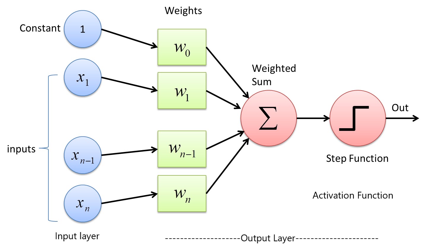
Input layer in above diagram takes data input, if n=10 then it is like there are 10 feature which are given as data input for model training or prediction. w0, w1, w2, etc are weight assigned for the each input, these weights are learned during the training process. These are same as b0, b1, b2 etc of classical machine learning. b0 or w0 can be considered as intercept by a hyperplane.
We know that a linear regerssion equation is like
$$y = w_0 + w_1x_1 + w_2x_2 + w_3x_3…… w_nx_n$$
Logistic regression equation is
$$y = \frac{1}{1-e^{-y}}$$
Activation function#
Activation functions are mathematical functions that are used in artificial neural networks to introduce non-linearity into the model. They are applied element-wise to the output of the dot product of the input and the weight matrix, and the result is passed to the next layer.
There are several commonly used activation functions, each with its own properties and suitability for different types of problems. Some of the most popular activation functions are:
Sigmodraft: false id: It produces an output between 0 and 1, which makes it useful for output layers in which the predictions are probabilities. However, it has a tendency to saturate and produce gradients close to zero or close to one when the input values are small or large, which can slow down training.
ReLU (Rectified Linear Unit): It computes the function f(x) = max(0,x). The output is between 0 and Max(x) It is widely used in neural networks because it is computationally efficient and helps to prevent the vanishing gradient problem. In all computer vision network this is used heavily in the hidden layers.
Tanh (hyperbolic tangent): It produces an output between -1 and 1, which makes it useful for output layers in which the predictions are normalized values. It is similar to sigmoid but it is zero-centered.
Leaky ReLU: This function is an extension of ReLU. It solves the dying ReLU problem by introducing a small slope for negative inputs.
Softmax: It is a generalization of the sigmoid function to multi-class classification problems. It maps the output of the last layer to a probability distribution over the classes.
$$\sigma(z_i) = \frac{e^{z_i}}{\sum_{j=1}^{n} e^{z_j}}$$
Where $z$ is the input vector to the activation function, $i$ is the index of the current neuron, and $n$ is the total number of neurons in the layer. The output of the softmax function, $\sigma(z_i)$, is a probability value between 0 and 1, and the sum of all the probability values for all the neurons in the layer is 1.
Activation functions are a crucial component of neural networks. They introduce non-linearity in the model, allowing the network to learn complex, non-linear relationships in the data. The choice of activation function depends on the problem, and often requires some experimentation to find the best one.
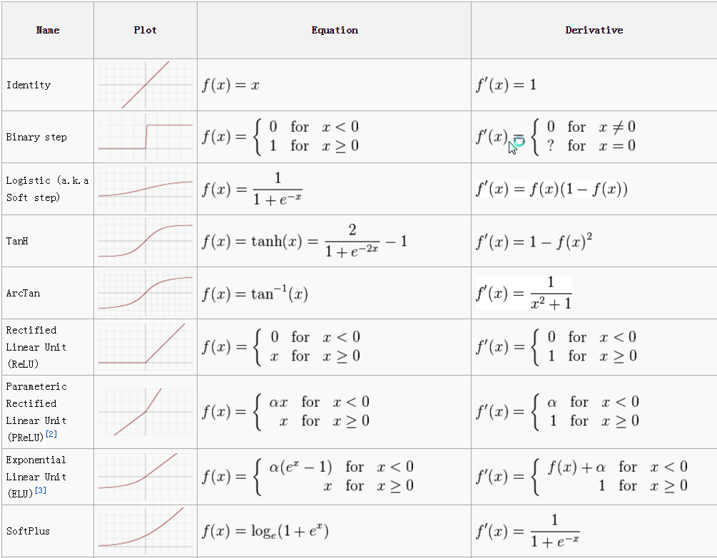
Image Credit
Assumptions of a neural network.#
Neural networks are a powerful tool for modeling complex systems, but they do have certain assumptions and limitations. Some of the main assumptions of neural networks are:
- Linearity: Neural networks are based on the assumption that the relationship between the input and output variables is linear. This assumption is relaxed by introducing non-linear activation functions in the model.
- Stationarity: Neural networks assume that the statistical properties of the data do not change over time. In other words, the model’s assumptions about the data distribution are fixed and do not change as the data is collected.
- Independence: Neural networks assume that the input variables are independent of each other, which means that the value of one variable does not depend on the value of the other variable. This assumption is relaxed by using techniques such as convolutional layers or recurrent layers to model dependencies between input variables.
- Large amount of data: Neural network requires a large amount of data for training. With a large amount of data, neural network can learn complex relationships and generalize well to unseen data.
- Structured Data: Neural networks assume that the data is structured in a way that allows it to learn meaningful patterns. This means that the data should be cleaned, normalized, and transformed as necessary to ensure that it can be used effectively by the model.
It’s important to note that these assumptions may not always hold, especially in real-world problems, and the model may not work well in such cases. Additionally, there are other assumptions which are specific to different types of neural networks, such as assumptions of linearity, sparsity, and stationarity in Autoencoder, assumptions of temporal dependencies in RNN (Recurrent Neural Networks).
Backpropagation using a simple example#
During Backpropagation, The weights of the network connections are repeatedly adjusted to minimize the difference between the actual output vector of the net and the desired output vector.
Neural Network using Tensorflow#
What is keras and how is it different from Tensorflow?#
Keras is a high-level Python deep learning library that simplifies the creation of deep learning models. It was initially developed as part of the TensorFlow library, but has since been separated into its own standalone library. Keras is designed to enable fast experimentation with deep neural networks and offers a simple interface for defining and training complex models. In comparison, TensorFlow is a low-level library that provides more control over the implementation of the deep learning model, but requires more configuration and coding.
What are Dense layers#
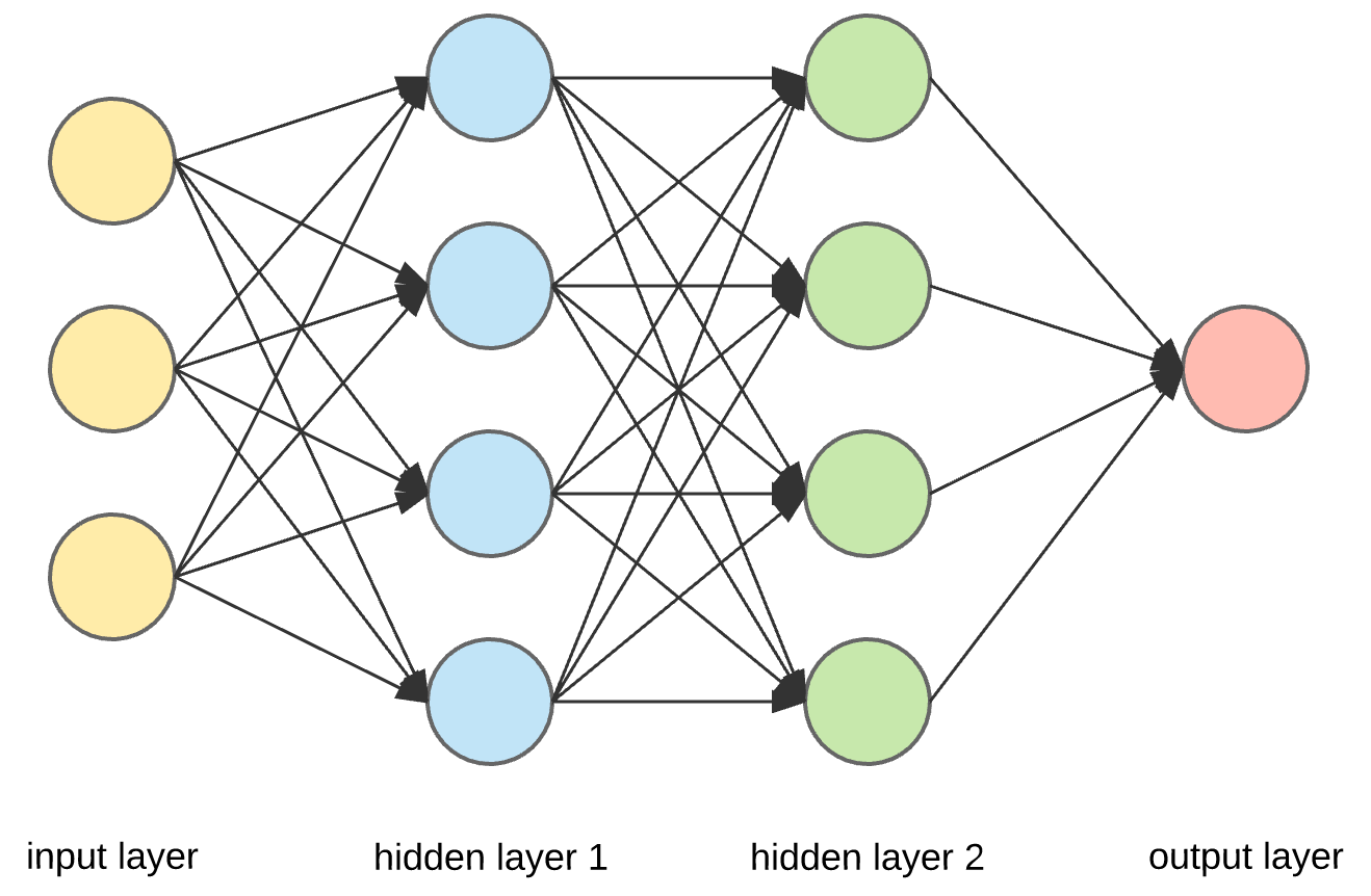
Dense layers, also known as fully connected layers, are a type of layer commonly used in neural networks. In a dense layer, every neuron in the layer is connected to every neuron in the previous layer, hence the name fully connected.
The dense layer takes an input vector and the output vector is obtained by computing a dot product of the input vector with a weight matrix, and adding a bias vector. This is followed by applying an activation function element-wise.
Dense layers are used to learn non-linear combinations of the input features and are the basic building blocks of a neural network. They can be stacked on top of each other to form a multi-layer perceptron, where the output of one dense layer is passed as input to the next dense layer. This allows the model to learn increasingly complex representations of the input data.
A dense layer can have any number of neurons, and the number of neurons in a dense layer determines the dimensionality of the output. The number of neurons in a dense layer can be used as a hyperparameter to control the capacity of the model.
In summary, Dense layers are a type of layer commonly used in neural networks. They are fully connected layers, where each neuron is connected to every neuron in the previous layer. They are used to learn non-linear combinations of the input features and are the basic building blocks of a neural network.

Comments: